Educational disclaimer. Service names, endpoints, caps and printed values are snapshots from the day this was written and will drift. Every number was measured on the free simulator tier, on one dataset, and does not transfer.
1. Shape the payload and the pools
Pull AI4I from OpenML, build the dict-of-dicts data.json the service actually reads, and put it in a data pool it can reach.
2. Run it and read what came back
A six-field request to the free Rimay simulator at 2,000 shots, then eleven quantum columns row-aligned with your original six.
3. Work out whether it helps
Keep the columns Fisher ranks worth keeping, read PR against ROC, score every row out of fold, then correct the significance test.
The business session closed on a four-step workflow. Today you run it on your own extraction:
| Workflow step from business session three | Lab steps |
|---|---|
| Plumbing, which the session did not show you | 0 setup, 1 payload, 2 pools, 3 extraction, 4 arrays |
| 1. Raw performance | 5: the progression, raw to expert to expert + Rimay |
| 2. Selection protocol | 5: gate the quantum columns against the classical scores |
| 3. Curve analysis | 6: precision-recall against ROC |
| 4. Significance | 7: out of fold, with the corrected p-values from Task 5 |
Each task carries a collapsed ladder: Hint 1 points at where to look, Hint 2 gives part of the answer, Solution gives all of it. Before you open any of them: what do you think is happening here?
Plumbing, Steps 0 to 4. Get your table into the service and the arrays back out.
Step 0: Set up the environment
Setup: uv project, SDKs, Hub credentials, .env
Python 3.11+, two Hub SDKs, three credentials.
uv init kipu-qml-lab
cd kipu-qml-lab
uv venv
uv add qhub-api qhub-service numpy pandas scikit-learn scipy matplotlib python-dotenv
Create an Application on the Hub dashboard, subscribe it to Rimay - Quantum Feature Extraction - Simulator on the Marketplace, FREE plan. Then a .env next to your scripts:
KQH_PERSONAL_ACCESS_TOKEN=...
KQH_ACCESS_KEY_ID=...
KQH_SECRET_ACCESS_KEY=...
| Variable | Where to get it |
|---|---|
KQH_PERSONAL_ACCESS_TOKEN | Settings, Personal Access Tokens |
KQH_ACCESS_KEY_ID | Applications, your application, Access Keys |
KQH_SECRET_ACCESS_KEY | Same place, shown once at creation |
A missing token surfaces as a bare 401 with an empty body on the first platform call; that means absent, not wrong.
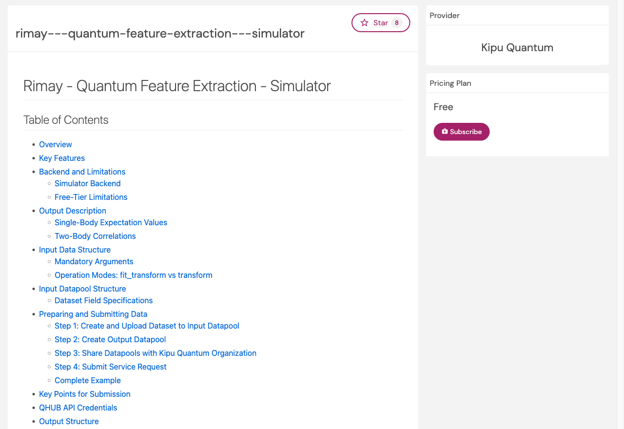
Free tier caps: 15 features, 3,000 samples across train and test. Everything here is sized to fit. Run scripts with uv run python task1_payload.py; Steps 1 and 5 to 8 are pure local Python, Steps 2 to 4 talk to the Hub.
Step 1: Get the data and shape the payload
The dataset is AI4I 2020, a public predictive-maintenance benchmark on OpenML: 10,000 machine records, 339 failures, five sensor readings plus a machine type code. You send nine features: those six plus three physics columns you derive here. The rest of the table is row ids and per-mode failure flags, and the flags are labels, so sending them would be leakage.
One extraction serves the whole lab: the raw-sensor baseline is a column subset, so Task 5 reads the whole progression off this run. What it cannot give you is a sensors-only quantum arm, because the circuit entangles all inputs. The business lesson measured that denied arm as its own submission and found nothing; carry that result with you, this lab does not re-measure it.
Task 1. Derive the three physics columns. The rest of the script is given.
You know the failure physics: heat dissipation fails when the process-to-air temperature difference is small, power failures when mechanical power (torque times angular speed) leaves its band, overstrain when tool wear times torque exceeds what the product type tolerates. Turn those three sentences into three columns:
# task1_payload.py: engineer the physics, build the 9-feature payload.
import json
import numpy as np
import pandas as pd
from sklearn.datasets import fetch_openml
from sklearn.model_selection import train_test_split
from sklearn.preprocessing import StandardScaler

df = fetch_openml("ai4i2020", version=1, as_frame=True).frame
df["type_code"] = df["Type"].map({"L": 0, "M": 1, "H": 2}).astype(float)

df["temp_diff"] = ...     # TODO
df["power"] = ...         # TODO
df["overstrain"] = ...    # TODO

# Column ORDER is the feature-to-qubit map and decides the pair topology.
CTRL9 = [
    "Air temperature [K]",
    "Process temperature [K]",
    "Rotational speed [rpm]",
    "Torque [Nm]",
    "Tool wear [min]",
    "temp_diff",
    "power",
    "overstrain",
    "type_code",
]

X = df[CTRL9].astype(float)
y = df["Machine failure"].astype(int)

# Keep every failure, subsample non-failures up to the 3000-row cap.
rng = np.random.RandomState(42)
pos = y[y == 1].index.to_numpy()                       # 339 rows
neg = rng.choice(y[y == 0].index.to_numpy(), 3000 - len(pos), replace=False)
keep = np.concatenate([pos, neg])
rng.shuffle(keep)

Xk, yk = X.loc[keep], y.loc[keep]
X_train, X_test, y_train, y_test = train_test_split(
    Xk, yk, test_size=0.2, random_state=42, stratify=yk
)

# Fit the scaler on the training rows only. Rimay applies its own minmax scaler
# on top, which is monotone per column, so this does not change the encoding.
sc = StandardScaler().fit(X_train)
X_train = pd.DataFrame(sc.transform(X_train), columns=CTRL9)
X_test = pd.DataFrame(sc.transform(X_test), columns=CTRL9)
y_train = pd.Series(y_train.to_numpy(), name="label")
y_test = pd.Series(y_test.to_numpy(), name="label")

payload = {
    "X_train": X_train.to_dict(),
    "y_train": y_train.to_frame("label").to_dict(),
    "X_test": X_test.to_dict(),
    "y_test": y_test.to_frame("label").to_dict(),
}

# Row keys must agree between the feature block and the label block, per split.
for xk_, yk_ in (("X_train", "y_train"), ("X_test", "y_test")):
    xkeys = list(next(iter(payload[xk_].values())).keys())
    assert list(payload[yk_]["label"].keys()) == xkeys, xk_
    for col in payload[xk_].values():
        assert list(col.keys()) == xkeys, xk_

with open("data.json", "w") as fh:
    json.dump(payload, fh)

print(len(X_train), len(X_test), X_train.shape[1], int(y_train.sum() + y_test.sum()))
Hint 1, where to look
Each engineered column is a function of two columns you already have:
- temperature difference:
df["Process temperature [K]"],df["Air temperature [K]"] - mechanical power (torque times angular speed):
df["Torque [Nm]"],df["Rotational speed [rpm]"] - overstrain:
df["Tool wear [min]"],df["Torque [Nm]"]
Constant factors wash out under the z-scaler.
Hint 2, two of the three
df["temp_diff"] = df["Process temperature [K]"] - df["Air temperature [K]"]
df["power"] = df["Torque [Nm]"] * df["Rotational speed [rpm]"] * 2 * np.pi / 60
df["overstrain"] = df["Tool wear [min]"] * df["Torque [Nm]"]
Solution
# task1_payload.py: engineer the physics, build the 9-feature payload.
import json
import numpy as np
import pandas as pd
from sklearn.datasets import fetch_openml
from sklearn.model_selection import train_test_split
from sklearn.preprocessing import StandardScaler

df = fetch_openml("ai4i2020", version=1, as_frame=True).frame
df["type_code"] = df["Type"].map({"L": 0, "M": 1, "H": 2}).astype(float)

# The three engineered features, straight from the AI4I failure-mode physics:
# heat dissipation fails on a small temperature difference, power failures on
# torque times angular speed outside a band, overstrain on tool wear times torque.
# Constant factors do not matter: the z-scaler below removes them and Rimay's
# own minmax scaler is monotone per column.
df["temp_diff"] = df["Process temperature [K]"] - df["Air temperature [K]"]
df["power"] = df["Torque [Nm]"] * df["Rotational speed [rpm]"] * 2 * np.pi / 60
df["overstrain"] = df["Tool wear [min]"] * df["Torque [Nm]"]

# Column ORDER is the feature-to-qubit map and decides the pair topology.
CTRL9 = [
    "Air temperature [K]",
    "Process temperature [K]",
    "Rotational speed [rpm]",
    "Torque [Nm]",
    "Tool wear [min]",
    "temp_diff",
    "power",
    "overstrain",
    "type_code",
]

X = df[CTRL9].astype(float)
y = df["Machine failure"].astype(int)

# Keep every failure, subsample non-failures up to the 3000-row cap.
rng = np.random.RandomState(42)
pos = y[y == 1].index.to_numpy()                       # 339 rows
neg = rng.choice(y[y == 0].index.to_numpy(), 3000 - len(pos), replace=False)
keep = np.concatenate([pos, neg])
rng.shuffle(keep)

Xk, yk = X.loc[keep], y.loc[keep]
X_train, X_test, y_train, y_test = train_test_split(
    Xk, yk, test_size=0.2, random_state=42, stratify=yk
)

# Fit the scaler on the training rows only. Rimay applies its own minmax scaler
# on top, which is monotone per column, so this does not change the encoding.
sc = StandardScaler().fit(X_train)
X_train = pd.DataFrame(sc.transform(X_train), columns=CTRL9)
X_test = pd.DataFrame(sc.transform(X_test), columns=CTRL9)
y_train = pd.Series(y_train.to_numpy(), name="label")
y_test = pd.Series(y_test.to_numpy(), name="label")

payload = {
    "X_train": X_train.to_dict(),
    "y_train": y_train.to_frame("label").to_dict(),
    "X_test": X_test.to_dict(),
    "y_test": y_test.to_frame("label").to_dict(),
}

# Row keys must agree between the feature block and the label block, per split.
for xk_, yk_ in (("X_train", "y_train"), ("X_test", "y_test")):
    xkeys = list(next(iter(payload[xk_].values())).keys())
    assert list(payload[yk_]["label"].keys()) == xkeys, xk_
    for col in payload[xk_].values():
        assert list(col.keys()) == xkeys, xk_

with open("data.json", "w") as fh:
    json.dump(payload, fh)

print(len(X_train), len(X_test), X_train.shape[1], int(y_train.sum() + y_test.sum()))
2400 600 9 339
2,400 training rows, 600 test rows, nine features, 339 failures, a prevalence of about 11.3% on each split. Column order matters: it is the feature-to-qubit map and decides which pair columns come back.
Step 2: Two data pools, one file, one permission
Rimay reads data.json out of one pool and writes its results into another; the request carries only the two pool ids. The input pool holds exactly one file, named data.json.
Task 2. Run the pool setup, then give the application write access to the output pool (run only, no code task in this step).
# task2_pools.py
import io, json, os
from dotenv import load_dotenv
from qhub.api.platform import HubPlatformClient

load_dotenv()
platform = HubPlatformClient(api_key=os.getenv("KQH_PERSONAL_ACCESS_TOKEN"))

input_dp = platform.data_pools.create_data_pool(name="Rimay Lab Input")
output_dp = platform.data_pools.create_data_pool(name="Rimay Lab Output")

# A reused input pool may already hold a data.json. Replace it rather than adding a second.
for f in platform.data_pools.get_data_pool_files(id=input_dp.id):
    if f.name == "data.json":
        platform.data_pools.delete_data_pool_file(id=input_dp.id, file_id=f.id)

body = open("data.json", "rb").read()
platform.data_pools.add_data_pool_file(
    id=input_dp.id, file=("data.json", io.BytesIO(body))
)

print("input ", input_dp.id)
print("output", output_dp.id)
print(f"uploaded data.json ({len(body) / 1024:.0f} KB)")
Solution, the write access
input  <your input pool uuid>
output <your output pool uuid>
uploaded data.json (767 KB)
Two ways, either is enough: share each pool with the Kipu Quantum organization at role MAINTAINER in the dashboard (Sharing tab), or send per-application grants with the Step 3 request (VIEW on input, MODIFY on output).
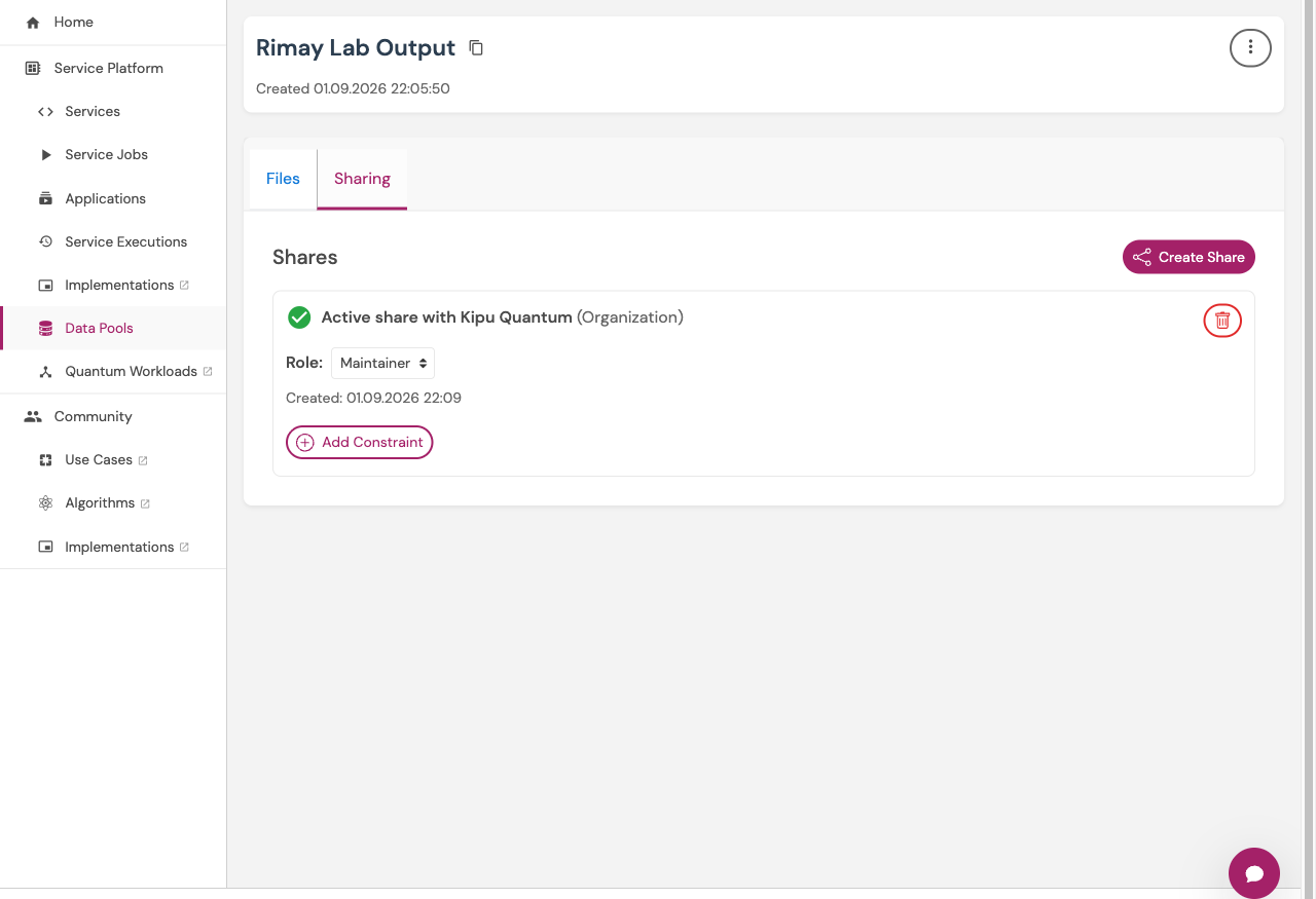
Caution. Insufficient write access on the output pool does not raise. The run reports SUCCEEDED and the output pool is empty. If you see that, fix the write access and resubmit.
Step 3: Run the extraction
Rimay runs on ibm_aer, the Qiskit Aer state-vector simulator, not a quantum processor. The request is six flat fields; three field names carry a leading underscore, which is part of the name, and _fit_reference wants the literal string "None". The script below carries all of that; run at 2,000 shots, because 500 shots produced a false null on this same table (+0.0151, p 0.25, against +0.0482 at p 2.5e-04 with 2,000).
Task 3. Submit. The only edit is pasting your two pool ids from Task 2.
# task3_submit.py
import os
import uuid
from dotenv import load_dotenv
from qhub.service.client import HubServiceClient

load_dotenv()

INPUT_POOL_ID = "paste-the-input-pool-id-task2-printed"
OUTPUT_POOL_ID = "paste-the-output-pool-id-task2-printed"

for _name, _val in (("INPUT_POOL_ID", INPUT_POOL_ID), ("OUTPUT_POOL_ID", OUTPUT_POOL_ID)):
    try:
        uuid.UUID(_val)
    except ValueError:
        raise SystemExit(f"{_name} is still the placeholder: Replace with the Pool-ID from Task 2")

service = HubServiceClient(
    service_endpoint=(
        "https://gateway.hub.kipu-quantum.com/kipu-quantum/"
        "rimay---quantum-feature-extraction---simulator/1.0.0"
    ),
    access_key_id=os.getenv("KQH_ACCESS_KEY_ID"),
    secret_access_key=os.getenv("KQH_SECRET_ACCESS_KEY"),
)

execution = service.run(request={
    "input_data_pool": {"id": INPUT_POOL_ID, "ref": "DATAPOOL"},
    "output_data_pool": {"id": OUTPUT_POOL_ID, "ref": "DATAPOOL"},
    "_mode": "fit_transform",   # fit on train, transform train and test in one run
    "_fit_reference": "None",   # the LITERAL STRING, not Python None; see the caution
    "num_shots": 2000,          # not 500: see the shot-count note above
    "num_runs": 1,
})

print("execution id:", execution.id)
execution.wait_for_final_state(timeout=900, wait=10)
print("status:", execution.status)

if execution.status == "FAILED":
    for log in execution.logs():
        print(log)
Expect a few minutes of queue and run time. A guard at the top fails loudly if you forgot the paste.
Step 4: Fetch the arrays
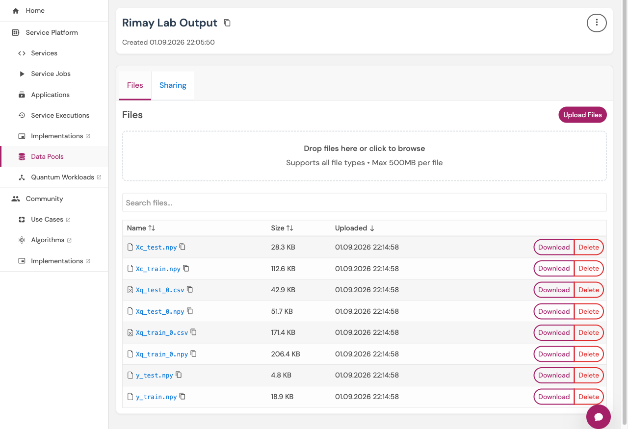
The output pool holds six .npy files: the classical block echoed back, the quantum block, and the labels, for train and test each, row-aligned.
Task 4. Download the arrays. The only edit is your output pool id.
# task4_fetch.py
import os
import uuid
import numpy as np
from pathlib import Path
from dotenv import load_dotenv
from qhub.api.platform import HubPlatformClient

load_dotenv()
platform = HubPlatformClient(api_key=os.getenv("KQH_PERSONAL_ACCESS_TOKEN"))

OUTPUT_POOL_ID = "paste-the-output-pool-id-task2-printed"

try:
    uuid.UUID(OUTPUT_POOL_ID)
except ValueError:
    raise SystemExit("OUTPUT_POOL_ID is still the placeholder: paste the id Task 2 printed")

out_dir = Path("rimay_output")
out_dir.mkdir(exist_ok=True)

def download_verified(dp_id, f, dest, attempts=3):
    """Stream a pool file and verify the full content_length actually arrived."""
    for attempt in range(1, attempts + 1):
        try:
            stream = platform.data_pools.get_data_pool_file(id=dp_id, file_id=f.id)
            n = 0
            with open(dest, "wb") as fp:
                for chunk in stream:
                    n += len(chunk)
                    fp.write(chunk)
            if f.content_length and n != f.content_length:
                raise IOError(f"received {n}/{f.content_length} bytes")
            return n
        except Exception as e:
            if attempt == attempts:
                raise RuntimeError(f"failed to download {f.name}: {e}") from e

for f in platform.data_pools.get_data_pool_files(id=OUTPUT_POOL_ID):
    if f.name.endswith(".npy"):
        n = download_verified(OUTPUT_POOL_ID, f, out_dir / f.name)
        print(f"  {f.name} ({n} bytes)")

Xc_train = np.load(out_dir / "Xc_train.npy")
Xq_train = np.load(out_dir / "Xq_train_0.npy")
n_c, n_q = Xc_train.shape[1], Xq_train.shape[1]
print(f"classical {n_c}, quantum {n_q} = {n_c} per-feature + {n_q - n_c} pairs")
assert n_q == 2 * n_c - 1
assert n_c == 9, "expected the 9-feature extraction; re-run Tasks 1 to 3"
classical 9, quantum 17 = 9 per-feature + 8 pairs
The width rule: 2n - 1 quantum columns for n input features, one per feature plus n - 1 data-driven pairs.
Workflow steps 1 and 2, Step 5. Raw performance, then the selection protocol.
Step 5: The progression, and the gate
From here everything is local Python, and the tasks share a module lab_common.py: this task starts it, Task 6 appends to it, Tasks 7 and 8 import from it.
The measurement is the progression raw, expert, expert + Rimay, each arm read against the arm it has to beat, with a Wilcoxon signed-rank p-value per step, Holm corrected within each model, under two protocols (15 random splits, and out-of-fold). The models are naive Bayes, logistic regression and linear SVM; RBF SVM and gradient boosting sit out for training time, and the study's readings for them are quoted after the solution.
Selection is the second half. The score is the Fisher discriminant: per column, squared class-mean gap over summed class variance, computed on the training fold only. The cutoff is not a fixed top-k but a knob, GATE_QUANTILE: a quantum column enters only if its score clears that quantile of the classical columns' own scores. At 0.5 a quantum column has to be at least as informative as the typical column you already had.
Task 5. Fill in the four arms, their baselines, and the gate quantile. The harness is given.
- Save the module below as
lab_common.pynext to your scripts. - In
task5_compare.py, provide the training features from Task 4's output at eachTODO: which columns form each arm, which arm it is read against, and the gate quantile.
lab_common.py, given, started here and grown in Task 6:
# lab_common.py, started in Task 5
import numpy as np
from pathlib import Path
from sklearn.base import BaseEstimator, TransformerMixin

import numpy as np
from pathlib import Path
from sklearn.base import BaseEstimator, TransformerMixin
from sklearn.pipeline import Pipeline
from sklearn.preprocessing import StandardScaler
from sklearn.model_selection import GridSearchCV, StratifiedKFold
from sklearn.naive_bayes import GaussianNB

# The raw sensor columns inside the 9-column table: five sensors plus type code.
RAW = [0, 1, 2, 3, 4, 8]

# Kipu brand colors (tokens.css)
GOLD, MUTED, FG, BG = "#b38f12", "#6b6b6b", "#0f1319", "#ffffff"

def load_arrays(out_dir="rimay_output"):
    """The six row-aligned arrays Task 4 downloaded, in one call."""
    d = Path(out_dir)
    return (np.load(d / "Xc_train.npy"), np.load(d / "Xq_train_0.npy"),
            np.load(d / "y_train.npy").ravel().astype(int),
            np.load(d / "Xc_test.npy"), np.load(d / "Xq_test_0.npy"),
            np.load(d / "y_test.npy").ravel().astype(int))

def fisher_scores(X, y):
    """Per-column Fisher ratio: squared class-mean gap over summed class variance."""
    a, b = X[y == 1], X[y == 0]
    return (a.mean(0) - b.mean(0))**2 / (a.var(0) + b.var(0) + 1e-12)

class FisherGate(BaseEstimator, TransformerMixin):
    """Adaptive cutoff instead of a fixed top-k. Keep all n_raw classical
    columns; keep a quantum column only if its Fisher score clears the median
    of the classical columns' own scores. In words: a quantum column has to be
    at least as informative, on its own, as a typical column you already had.
    Computed inside fit, so it sees the training fold only."""
    def __init__(self, n_raw=9, q=0.5):
        self.n_raw, self.q = n_raw, q
    def fit(self, X, y):
        f = fisher_scores(X, y)
        thr = np.quantile(f[:self.n_raw], self.q)
        self.keep_ = np.r_[np.arange(self.n_raw),
                           self.n_raw + np.where(f[self.n_raw:] >= thr)[0]]
        return self
    def transform(self, X):
        return X[:, self.keep_]
The harness, fill the arms:
# task5_compare.py: the progression, raw -> expert -> expert + Rimay.
import numpy as np
from scipy.stats import wilcoxon
from sklearn.base import clone
from sklearn.pipeline import Pipeline
from sklearn.preprocessing import StandardScaler
from sklearn.model_selection import StratifiedKFold, GridSearchCV
from sklearn.naive_bayes import GaussianNB
from sklearn.model_selection import StratifiedShuffleSplit, RepeatedStratifiedKFold
from sklearn.metrics import average_precision_score
from sklearn.linear_model import LogisticRegression
from sklearn.svm import LinearSVC
from lab_common import load_arrays, FisherGate, RAW

# RBF SVM and gradient boosting sit out of this panel for training time; the
# study's Holm-corrected readings for both are quoted below the expected output.
MODELS = {
    "naive bayes":         (GaussianNB(), {"m__var_smoothing": [1e-9, 1e-7, 1e-5, 1e-3]}),
    "logistic regression": (LogisticRegression(max_iter=5000), {"m__C": [0.01, 0.1, 1, 10, 100]}),
    "linear SVM":          (LinearSVC(max_iter=20000, dual="auto"), {"m__C": [0.01, 0.1, 1, 10]}),
}

def holm(pvals):
    """Holm step-down correction over a dict of name -> raw p-value."""
    items = sorted(pvals.items(), key=lambda kv: kv[1])
    m, out, running = len(items), {}, 0.0
    for i, (name, p) in enumerate(items):
        running = max(running, (m - i) * p)
        out[name] = min(1.0, running)
    return out

Xc_train, Xq_train, y_train, Xc_validate, Xq_validate, y_validate = load_arrays()
Xc = np.vstack([Xc_train, Xc_validate])
Xq = np.vstack([Xq_train, Xq_validate])
Y = np.concatenate([y_train, y_validate])
assert Xc.shape[1] == 9, "rimay_output holds an older run; re-run Tasks 1 to 4"

# The progression: each arm is read against the one it has to beat.
# TODO: the gate's knob. A quantum column must clear this quantile of the
# classical columns' own Fisher scores. Where does a quantum column earn its
# place: above the weakest classical column, the typical one, the best one?
GATE_QUANTILE = ...

ARMS = {
    "raw":          (Xc[:, RAW], None),   # sensors only, no extraction needed
    "expert":       (..., None),          # TODO: which columns?
    "expert+all":   (..., None),          # TODO: which columns?
    "expert+gated": (..., FisherGate(q=GATE_QUANTILE)),  # TODO: which columns feed the gate?
}
# TODO: each arm is read against the arm it has to beat. Which one is that?
BASELINE = {"expert": ..., "expert+all": ..., "expert+gated": ...}

def fit_score(X, est, grid, sel, tr, te, seed):
    steps = [("sc", StandardScaler())]
    if sel is not None:
        steps.insert(0, ("sel", clone(sel)))
    steps.append(("m", clone(est)))
    gs = GridSearchCV(Pipeline(steps), grid, scoring="average_precision",
                      cv=StratifiedKFold(3, shuffle=True, random_state=seed), n_jobs=1)
    gs.fit(X[tr], Y[tr])
    b = gs.best_estimator_
    s = (b.decision_function(X[te]) if hasattr(b, "decision_function")
         else b.predict_proba(X[te])[:, 1])
    return average_precision_score(Y[te], s)

# Two evaluation protocols over the same arms. split: 15 random 80/20 draws.
# oof: 5 folds x 3 repeats, every row tested exactly once per repeat, the
# fold-level pairing the Step 7 curves argue for.
PROTOCOLS = {
    "split": list(StratifiedShuffleSplit(n_splits=15, test_size=0.2,
                                         random_state=7).split(Xc, Y)),
    "oof":   list(RepeatedStratifiedKFold(n_splits=5, n_repeats=3,
                                          random_state=7).split(Xc, Y)),
}

res = {}
for proto, splits in PROTOCOLS.items():
    out = {(m, a): [] for m in MODELS for a in ARMS}
    for seed, (tr, te) in enumerate(splits):
        for m, (est, grid) in MODELS.items():
            for a, (X, sel) in ARMS.items():
                out[(m, a)].append(fit_score(X, est, grid, sel, tr, te, seed))
    res[proto] = out

# Absolute AP per arm, delta against the arm's own baseline, and a Wilcoxon
# signed-rank p per step, Holm corrected across the three comparisons within
# each model, once per protocol.
for m in MODELS:
    ph = {}
    for proto in ("split", "oof"):
        ph[proto] = holm({a: wilcoxon(np.array(res[proto][(m, a)]),
                                      np.array(res[proto][(m, BASELINE[a])])).pvalue
                          for a in BASELINE})
    line = f"{m:20s} raw {np.mean(res['split'][(m, 'raw')]):.4f}"
    for a in ("expert", "expert+all", "expert+gated"):
        v = np.mean(res["split"][(m, a)])
        d = v - np.mean(res["split"][(m, BASELINE[a])])
        line += (f" | {a} {v:.4f} ({d:+.4f} vs {BASELINE[a]},"
                 f" p {ph['split'][a]:.4f}, oof p {ph['oof'][a]:.4f})")
    print(line)
Hint 1, where to look
Everything comes out of load_arrays(), which reads the six .npy files Task 4 downloaded into rimay_output/. Xc is the classical block the service echoed back, all nine columns in your Task 1 order; RAW (from lab_common) indexes the six sensor columns inside it; Xq is the seventeen quantum columns. An arm is a column stack: Xc[:, RAW] is sensors only, Xc is the engineered table, np.hstack([Xc, Xq]) appends the quantum block. Each arm's baseline is the previous step of the progression, by name in BASELINE. The gate quantile is where the spectrum plot draws its dashed line.
Hint 2, the arms
GATE_QUANTILE = 0.5

ARMS = {
    "raw":          (Xc[:, RAW], None),
    "expert":       (Xc, None),
    "expert+all":   (np.hstack([Xc, Xq]), None),
    "expert+gated": (np.hstack([Xc, Xq]), FisherGate(q=GATE_QUANTILE)),
}
BASELINE = {"expert": "raw", "expert+all": "expert", "expert+gated": "expert"}
The gated arm stacks the same columns as expert+all; the gate prunes inside the pipeline. 0.5 is the classical median; the solution shows the whole sweep so you can play with it.
Solution
The completed harness:
# task5_compare.py: the progression, raw -> expert -> expert + Rimay.
import numpy as np
from scipy.stats import wilcoxon
from sklearn.base import clone
from sklearn.model_selection import StratifiedShuffleSplit, RepeatedStratifiedKFold
from sklearn.metrics import average_precision_score
from sklearn.linear_model import LogisticRegression
from sklearn.svm import LinearSVC
from sklearn.pipeline import Pipeline
from sklearn.preprocessing import StandardScaler
from sklearn.model_selection import StratifiedKFold, GridSearchCV
from sklearn.naive_bayes import GaussianNB
from lab_common import load_arrays, FisherGate, RAW

# RBF SVM and gradient boosting sit out of this panel for training time; the
# study's Holm-corrected readings for both are quoted below the expected output.
MODELS = {
    "naive bayes":         (GaussianNB(), {"m__var_smoothing": [1e-9, 1e-7, 1e-5, 1e-3]}),
    "logistic regression": (LogisticRegression(max_iter=5000), {"m__C": [0.01, 0.1, 1, 10, 100]}),
    "linear SVM":          (LinearSVC(max_iter=20000, dual="auto"), {"m__C": [0.01, 0.1, 1, 10]}),
}

def holm(pvals):
    """Holm step-down correction over a dict of name -> raw p-value."""
    items = sorted(pvals.items(), key=lambda kv: kv[1])
    m, out, running = len(items), {}, 0.0
    for i, (name, p) in enumerate(items):
        running = max(running, (m - i) * p)
        out[name] = min(1.0, running)
    return out

Xc_train, Xq_train, y_train, Xc_validate, Xq_validate, y_validate = load_arrays()
Xc = np.vstack([Xc_train, Xc_validate])
Xq = np.vstack([Xq_train, Xq_validate])
Y = np.concatenate([y_train, y_validate])
assert Xc.shape[1] == 9, "rimay_output holds an older run; re-run Tasks 1 to 4"

# The progression: each arm is read against the one it has to beat.
# The gate's knob: a quantum column must clear this quantile of the classical
# columns' own Fisher scores. 0.5 = at least as good as the typical column.
GATE_QUANTILE = 0.5

ARMS = {
    "raw":          (Xc[:, RAW], None),                # sensors only, no extraction needed
    "expert":       (Xc, None),                        # + the three engineered columns
    "expert+all":   (np.hstack([Xc, Xq]), None),       # + all 17 quantum columns
    "expert+gated": (np.hstack([Xc, Xq]), FisherGate(q=GATE_QUANTILE)),
}
BASELINE = {"expert": "raw", "expert+all": "expert", "expert+gated": "expert"}

def fit_score(X, est, grid, sel, tr, te, seed):
    steps = [("sc", StandardScaler())]
    if sel is not None:
        steps.insert(0, ("sel", clone(sel)))
    steps.append(("m", clone(est)))
    gs = GridSearchCV(Pipeline(steps), grid, scoring="average_precision",
                      cv=StratifiedKFold(3, shuffle=True, random_state=seed), n_jobs=1)
    gs.fit(X[tr], Y[tr])
    b = gs.best_estimator_
    s = (b.decision_function(X[te]) if hasattr(b, "decision_function")
         else b.predict_proba(X[te])[:, 1])
    return average_precision_score(Y[te], s)

# Two evaluation protocols over the same arms. split: 15 random 80/20 draws.
# oof: 5 folds x 3 repeats, every row tested exactly once per repeat, the
# fold-level pairing the Step 7 curves argue for.
PROTOCOLS = {
    "split": list(StratifiedShuffleSplit(n_splits=15, test_size=0.2,
                                         random_state=7).split(Xc, Y)),
    "oof":   list(RepeatedStratifiedKFold(n_splits=5, n_repeats=3,
                                          random_state=7).split(Xc, Y)),
}

res = {}
for proto, splits in PROTOCOLS.items():
    out = {(m, a): [] for m in MODELS for a in ARMS}
    for seed, (tr, te) in enumerate(splits):
        for m, (est, grid) in MODELS.items():
            for a, (X, sel) in ARMS.items():
                out[(m, a)].append(fit_score(X, est, grid, sel, tr, te, seed))
    res[proto] = out

# Absolute AP per arm, delta against the arm's own baseline, and a Wilcoxon
# signed-rank p per step, Holm corrected across the three comparisons within
# each model, once per protocol.
for m in MODELS:
    ph = {}
    for proto in ("split", "oof"):
        ph[proto] = holm({a: wilcoxon(np.array(res[proto][(m, a)]),
                                      np.array(res[proto][(m, BASELINE[a])])).pvalue
                          for a in BASELINE})
    line = f"{m:20s} raw {np.mean(res['split'][(m, 'raw')]):.4f}"
    for a in ("expert", "expert+all", "expert+gated"):
        v = np.mean(res["split"][(m, a)])
        d = v - np.mean(res["split"][(m, BASELINE[a])])
        line += (f" | {a} {v:.4f} ({d:+.4f} vs {BASELINE[a]},"
                 f" p {ph['split'][a]:.4f}, oof p {ph['oof'][a]:.4f})")
    print(line)
And the spectrum plot, task5b_spectrum.py:
# task5b_spectrum.py: what the gate sees. Fisher scores of all 26 columns,
# computed on the training split only, classical vs quantum, threshold marked.
import numpy as np
import matplotlib.pyplot as plt
from lab_common import load_arrays, fisher_scores, GOLD, MUTED, FG, BG

Xc_train, Xq_train, y_train, *_ = load_arrays()
X = np.hstack([Xc_train, Xq_train])
f = fisher_scores(X, y_train)
n_raw = Xc_train.shape[1]
GATE_QUANTILE = 0.5
thr = np.quantile(f[:n_raw], GATE_QUANTILE)

names = ([f"c{i}" for i in range(n_raw)]
         + [f"q{i}" for i in range(n_raw)]
         + [f"pair{i}" for i in range(X.shape[1] - 2 * n_raw)])
order = np.argsort(-f)

fig, ax = plt.subplots(figsize=(14, 5), dpi=100)
fig.patch.set_facecolor(BG)
colors = [FG if i < n_raw else GOLD for i in order]
ax.bar(range(len(f)), f[order], color=colors)
ax.axhline(thr, color=MUTED, lw=1.5, ls="--")
ax.text(len(f) - 0.5, thr, "  gate threshold: q-quantile of the classical scores", color=MUTED,
        va="bottom", ha="right", fontsize=9, fontfamily="monospace")
ax.set_xticks(range(len(f)))
ax.set_xticklabels([names[i] for i in order], rotation=60, fontsize=8,
                   fontfamily="monospace")
ax.set_ylabel("FISHER SCORE")
ax.set_title("The spectrum the gate cuts: classical (dark) vs quantum (gold)",
             color=FG, fontweight="bold", loc="left")
ax.set_facecolor(BG)
for sp in ("top", "right"): ax.spines[sp].set_visible(False)
for sp in ("left", "bottom"): ax.spines[sp].set_color(MUTED)
ax.yaxis.label.set_fontfamily("monospace"); ax.yaxis.label.set_color(MUTED)
ax.tick_params(colors=MUTED)
fig.tight_layout()
fig.savefig("fisher-scores.png", facecolor=BG, bbox_inches="tight")
plt.show()

kept = int((f[n_raw:] >= thr).sum())
print(f"threshold {thr:.4f} (q={GATE_QUANTILE} quantile of the {n_raw} classical scores)")
print(f"quantum columns kept: {kept} of {X.shape[1] - n_raw}")
print("top five columns:", ", ".join(f"{names[i]} {f[i]:.3f}" for i in order[:5]))
The script's actual output on the verified arrays, run 8 September 2026:
naive bayes          raw 0.5487 | expert 0.6650 (+0.1163 vs raw, p 0.0002, oof p 0.0002) | expert+all 0.7232 (+0.0582 vs expert, p 0.0002, oof p 0.0002) | expert+gated 0.7296 (+0.0646 vs expert, p 0.0002, oof p 0.0002)
logistic regression  raw 0.6560 | expert 0.6985 (+0.0424 vs raw, p 0.0004, oof p 0.0009) | expert+all 0.7447 (+0.0463 vs expert, p 0.0002, oof p 0.0012) | expert+gated 0.7225 (+0.0240 vs expert, p 0.0012, oof p 0.0054)
linear SVM           raw 0.6602 | expert 0.7031 (+0.0429 vs raw, p 0.0006, oof p 0.0005) | expert+all 0.7451 (+0.0420 vs expert, p 0.0002, oof p 0.0006) | expert+gated 0.7236 (+0.0205 vs expert, p 0.0012, oof p 0.0009)
Every step of the progression is significant, under both protocols, for all three models. The gate helps the one model that cannot ignore a column (naive Bayes: gated +0.0646 beats unselected +0.0582) and costs the two linear models, which down-weight weak columns on their own. Selection is a property of the receiving model, not of the columns.
The knob, swept (delta vs expert, 15-split means; kept = quantum columns surviving of 17):
q      kept   naive bayes   logistic regression   linear SVM
0.00   14.9     +0.0583          +0.0274           +0.0245
0.25   14.0     +0.0591          +0.0254           +0.0230
0.50    7.9     +0.0646          +0.0240           +0.0205
0.75    3.1     +0.0369          +0.0249           +0.0209
1.00    3.0     +0.0359          +0.0257           +0.0216
For naive Bayes the ridge peaks at the median; the linear models are nearly flat and slightly prefer keeping more. No single q is "best": the receiving model decides, which is the capacity statement in one table.
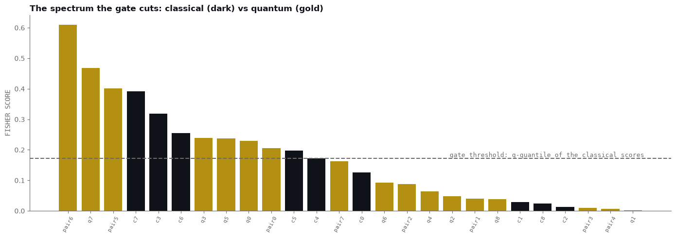
The spectrum shows why the rule is what it is: the top of it is quantum (a pair column at 0.61 beats the best classical column at 0.39), and the scores decay smoothly with no junk block to cut at, so the threshold is anchored to the classical scores instead of eyeballed.
Three boundaries travel with the positive, all from the study behind this page:
- Re-presentation, not discovery. The sensors-only extraction moved no model significantly; the gain appears only when the physics is already in the payload.
- The strong models go the other way. RBF SVM loses -0.0506 and gradient boosting -0.0476 against the engineered table, both significant, and gradient boosting on the engineered table alone stands at 0.9420 average precision, above every quantum arm.
- AI4I is the only gainer of four datasets tested. Pima, UNSW and Cleveland showed nothing.
Caution. Fisher score computed on the whole dataset and then used to select is leakage. The gate computes it inside
fit, on the training fold only; that distinction is invisible in the printed number and decisive in whether it means anything.
Workflow step 3, Step 6. Read the result on the curve.
Step 6: Read the result on the curve your stakeholder lives on
ROC divides false alarms by the healthy machines, of which there are eight times more than failures here; PR divides them by the alarms themselves. The rarer and more expensive the positive class, the more the PR curve is the picture you want, and average precision is its one-number summary. Chance is the diagonal on ROC and the prevalence line on PR.
Task 6. Fill in the three curves. The plotting is given.
First append the tuned pipeline to lab_common.py, given:
# lab_common.py, appended in Task 6
from sklearn.pipeline import Pipeline
from sklearn.preprocessing import StandardScaler
from sklearn.model_selection import GridSearchCV, StratifiedKFold
from sklearn.naive_bayes import GaussianNB

def nb_search(seed, gate=False, n_jobs=1):
    """The Task 5 naive-Bayes protocol as one reusable estimator: scaler plus
    GaussianNB, smoothing grid chosen by inner CV, optionally behind the
    FisherGate. Steps 6 to 8 reuse it."""
    steps = [("sc", StandardScaler()), ("m", GaussianNB())]
    if gate:
        steps.insert(0, ("sel", FisherGate()))
    grid = {"m__var_smoothing": [1e-9, 1e-7, 1e-5, 1e-3]}
    return GridSearchCV(Pipeline(steps), grid, scoring="average_precision",
                        cv=StratifiedKFold(3, shuffle=True, random_state=seed),
                        n_jobs=n_jobs)
Then fill the curves:
# task6_prcurve.py: ROC and PR for the progression, one model, three arms.
import numpy as np
import matplotlib.pyplot as plt
from sklearn.metrics import (precision_recall_curve, roc_curve,
                             average_precision_score, roc_auc_score)
from lab_common import load_arrays, nb_search, RAW, GOLD, MUTED, FG, BG

Xc_train, Xq_train, y_train, Xc_validate, Xq_validate, y_validate = load_arrays()
assert Xc_train.shape[1] == 9, "rimay_output holds an older run; re-run Tasks 1 to 4"

def fit_score(Xtr, Xte, gate=False):
    gs = nb_search(seed=0, gate=gate)
    gs.fit(Xtr, y_train)
    return gs.best_estimator_.predict_proba(Xte)[:, 1]

# The extraction already handed you one fixed split: 2,400 train, 600 validation.
CURVES = [
    # TODO: three (name, color, scores) entries, the progression from Task 5:
    # raw 6 in MUTED, expert 9 in FG, expert + Rimay (gated) in GOLD
]

fig, (axr, axp) = plt.subplots(1, 2, figsize=(14, 6), dpi=100)
fig.patch.set_facecolor(BG)
prev = y_validate.mean()

for name, col, s in CURVES:
    fpr, tpr, _ = roc_curve(y_validate, s)
    axr.plot(fpr, tpr, color=col, lw=3, solid_capstyle="round",
             label=f"{name}  AUC {roc_auc_score(y_validate, s):.3f}")
    p, r, _ = precision_recall_curve(y_validate, s)
    axp.plot(r, p, color=col, lw=3, solid_capstyle="round",
             label=f"{name}  AP {average_precision_score(y_validate, s):.3f}")

axr.plot([0, 1], [0, 1], color=MUTED, lw=1, ls="--")           # chance: the diagonal
axp.axhline(prev, color=MUTED, lw=1, ls="--")                  # chance: the prevalence
axr.set_xlabel("FALSE POSITIVE RATE"); axr.set_ylabel("TRUE POSITIVE RATE")
axp.set_xlabel("RECALL"); axp.set_ylabel("PRECISION")
axr.set_title("ROC: the gaps compress", color=FG, fontweight="bold", loc="left")
axp.set_title("PR: the picture your stakeholder lives in", color=FG, fontweight="bold", loc="left")
for ax in (axr, axp):
    ax.set_facecolor(BG)
    for sp in ("top", "right"): ax.spines[sp].set_visible(False)
    for sp in ("left", "bottom"): ax.spines[sp].set_color(MUTED)
    ax.xaxis.label.set_fontfamily("monospace"); ax.yaxis.label.set_fontfamily("monospace")
    ax.xaxis.label.set_color(MUTED); ax.yaxis.label.set_color(MUTED)
    ax.tick_params(colors=MUTED)
    ax.set_xlim(0, 1); ax.set_ylim(0, 1.02)
    ax.legend(frameon=False, fontsize=9, loc="lower right")
fig.tight_layout()
fig.savefig("pr-vs-roc.png", facecolor=BG, bbox_inches="tight")
plt.show()

print(f"prevalence {prev:.3f}, positives in validation {int(y_validate.sum())}")
for name, _, s in CURVES:
    print(f"{name:24s} ROC AUC {roc_auc_score(y_validate, s):.4f}"
          f"  AP {average_precision_score(y_validate, s):.4f}")
Hint 1, the first curve
("raw 6", MUTED, fit_score(Xc_train[:, RAW], Xc_validate[:, RAW])),
Hint 2, all three
CURVES = [
    ("raw 6",                  MUTED, fit_score(Xc_train[:, RAW], Xc_validate[:, RAW])),
    ("expert 9",               FG,    fit_score(Xc_train, Xc_validate)),
    ("expert + Rimay (gated)", GOLD,  fit_score(np.hstack([Xc_train, Xq_train]),
                                                np.hstack([Xc_validate, Xq_validate]), gate=True)),
]
Solution
# task6_prcurve.py: ROC and PR for the progression, one model, three arms.
import numpy as np
import matplotlib.pyplot as plt
from sklearn.metrics import (precision_recall_curve, roc_curve,
                             average_precision_score, roc_auc_score)
from lab_common import load_arrays, nb_search, RAW, GOLD, MUTED, FG, BG

Xc_train, Xq_train, y_train, Xc_validate, Xq_validate, y_validate = load_arrays()
assert Xc_train.shape[1] == 9, "rimay_output holds an older run; re-run Tasks 1 to 4"

def fit_score(Xtr, Xte, gate=False):
    gs = nb_search(seed=0, gate=gate)
    gs.fit(Xtr, y_train)
    return gs.best_estimator_.predict_proba(Xte)[:, 1]

# The extraction already handed you one fixed split: 2,400 train, 600 validation.
CURVES = [
    ("raw 6",                  MUTED, fit_score(Xc_train[:, RAW], Xc_validate[:, RAW])),
    ("expert 9",               FG,    fit_score(Xc_train, Xc_validate)),
    ("expert + Rimay (gated)", GOLD,  fit_score(np.hstack([Xc_train, Xq_train]),
                                                np.hstack([Xc_validate, Xq_validate]), gate=True)),
]

fig, (axr, axp) = plt.subplots(1, 2, figsize=(14, 6), dpi=100)
fig.patch.set_facecolor(BG)
prev = y_validate.mean()

for name, col, s in CURVES:
    fpr, tpr, _ = roc_curve(y_validate, s)
    axr.plot(fpr, tpr, color=col, lw=3, solid_capstyle="round",
             label=f"{name}  AUC {roc_auc_score(y_validate, s):.3f}")
    p, r, _ = precision_recall_curve(y_validate, s)
    axp.plot(r, p, color=col, lw=3, solid_capstyle="round",
             label=f"{name}  AP {average_precision_score(y_validate, s):.3f}")

axr.plot([0, 1], [0, 1], color=MUTED, lw=1, ls="--")           # chance: the diagonal
axp.axhline(prev, color=MUTED, lw=1, ls="--")                  # chance: the prevalence
axr.set_xlabel("FALSE POSITIVE RATE"); axr.set_ylabel("TRUE POSITIVE RATE")
axp.set_xlabel("RECALL"); axp.set_ylabel("PRECISION")
axr.set_title("ROC: the gaps compress", color=FG, fontweight="bold", loc="left")
axp.set_title("PR: the picture your stakeholder lives in", color=FG, fontweight="bold", loc="left")
for ax in (axr, axp):
    ax.set_facecolor(BG)
    for sp in ("top", "right"): ax.spines[sp].set_visible(False)
    for sp in ("left", "bottom"): ax.spines[sp].set_color(MUTED)
    ax.xaxis.label.set_fontfamily("monospace"); ax.yaxis.label.set_fontfamily("monospace")
    ax.xaxis.label.set_color(MUTED); ax.yaxis.label.set_color(MUTED)
    ax.tick_params(colors=MUTED)
    ax.set_xlim(0, 1); ax.set_ylim(0, 1.02)
    ax.legend(frameon=False, fontsize=9, loc="lower right")
fig.tight_layout()
fig.savefig("pr-vs-roc.png", facecolor=BG, bbox_inches="tight")
plt.show()

print(f"prevalence {prev:.3f}, positives in validation {int(y_validate.sum())}")
for name, _, s in CURVES:
    print(f"{name:24s} ROC AUC {roc_auc_score(y_validate, s):.4f}"
          f"  AP {average_precision_score(y_validate, s):.4f}")
prevalence 0.113, positives in validation 68
raw 6                    ROC AUC 0.8977  AP 0.5528
expert 9                 ROC AUC 0.9254  AP 0.6909
expert + Rimay (gated)   ROC AUC 0.9260  AP 0.7239
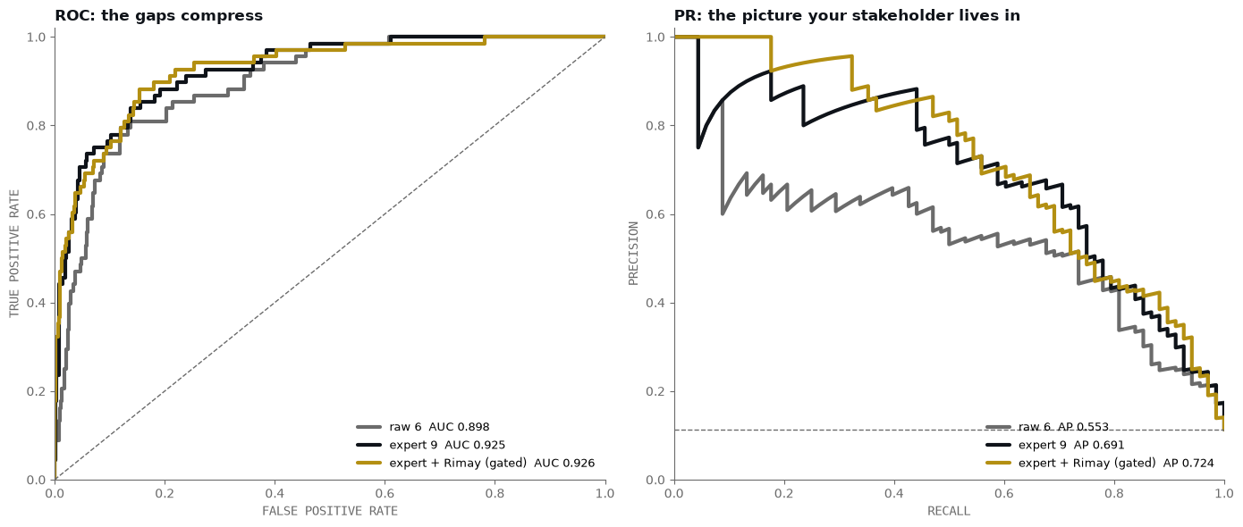
The expert and hybrid ROC curves lie on top of each other, AUC 0.9254 against 0.9260; the same two score vectors are +0.033 apart in AP. A real improvement in the region your application operates in, the top of the ranking, can be invisible on ROC, because ROC compresses exactly that region.
Workflow step 4, Step 7. Score every row you hold.
Step 7: Score every row: out-of-fold analysis
A single 80/20 split tests you on 600 rows and 68 failures; the rest of your data trains and never gets measured. Out-of-fold prediction recovers it: split into k folds, train on k-1, score the held-out fold, so every row is scored exactly once by a model that never saw it. Repeats with different fold assignments smooth where the boundaries fell.
Task 7. Choose the fold and repeat counts. The machinery is given.
# task7_oof_pr.py: the same comparison scored two ways.
import numpy as np
import matplotlib.pyplot as plt
from sklearn.model_selection import RepeatedStratifiedKFold
from sklearn.metrics import precision_recall_curve, average_precision_score
from lab_common import load_arrays, nb_search, GOLD, MUTED, FG, BG

Xc_train, Xq_train, y_train, Xc_validate, Xq_validate, y_validate = load_arrays()

# Pool the split back together: out-of-fold scores every one of the 3,000 rows.
Xc = np.vstack([Xc_train, Xc_validate])
Xq = np.vstack([Xq_train, Xq_validate])
Y = np.concatenate([y_train, y_validate])
X_hyb = np.hstack([Xc, Xq])

N_SPLITS = ...    # TODO: how many folds, so that every fold still holds enough failures?
N_REPEATS = ...   # TODO: how many repeats, to smooth where the fold boundaries fell?

def oof_scores(X, gate=False):
    """Every row scored N_REPEATS times by a model that never saw it."""
    acc, cnt = np.zeros(len(Y)), np.zeros(len(Y))
    rkf = RepeatedStratifiedKFold(n_splits=N_SPLITS, n_repeats=N_REPEATS, random_state=7)
    for tr, te in rkf.split(X, Y):
        gs = nb_search(seed=7, gate=gate, n_jobs=6)
        gs.fit(X[tr], Y[tr])
        acc[te] += gs.best_estimator_.predict_proba(X[te])[:, 1]
        cnt[te] += 1
    assert cnt.min() == N_REPEATS
    return acc / cnt

def single_split_scores(X_tr, X_te, gate=False):
    """The one fixed split the extraction handed you: 2,400 train, 600 validation."""
    gs = nb_search(seed=0, gate=gate)
    gs.fit(X_tr, y_train)
    return gs.best_estimator_.predict_proba(X_te)[:, 1]

panels = [
    ("One fixed split, 600 rows", y_validate,
     [("expert 9", FG, single_split_scores(Xc_train, Xc_validate)),
      ("expert + Rimay (gated)", GOLD,
       single_split_scores(np.hstack([Xc_train, Xq_train]),
                           np.hstack([Xc_validate, Xq_validate]), gate=True))]),
    ("Out of fold, all 3,000 rows", Y,
     [("expert 9", FG, oof_scores(Xc)),
      ("expert + Rimay (gated)", GOLD, oof_scores(X_hyb, gate=True))]),
]

fig, axes = plt.subplots(1, 2, figsize=(14, 6), dpi=100)
fig.patch.set_facecolor(BG)
for ax, (title, y_true, curves) in zip(axes, panels):
    for name, col, s in curves:
        p, r, _ = precision_recall_curve(y_true, s)
        ax.plot(r, p, color=col, lw=3, solid_capstyle="round",
                label=f"{name}  AP {average_precision_score(y_true, s):.3f}")
    ax.axhline(y_true.mean(), color=MUTED, lw=1, ls="--")
    ax.set_facecolor(BG)
    for sp in ("top", "right"): ax.spines[sp].set_visible(False)
    for sp in ("left", "bottom"): ax.spines[sp].set_color(MUTED)
    ax.set_xlabel("RECALL"); ax.set_ylabel("PRECISION")
    ax.xaxis.label.set_fontfamily("monospace"); ax.yaxis.label.set_fontfamily("monospace")
    ax.xaxis.label.set_color(MUTED); ax.yaxis.label.set_color(MUTED)
    ax.tick_params(colors=MUTED)
    ax.set_xlim(0, 1); ax.set_ylim(0, 1.02)
    ax.set_title(title, color=FG, fontweight="bold", loc="left")
    ax.legend(frameon=False, fontsize=9, loc="lower left")
fig.tight_layout()
fig.savefig("pr-single-vs-oof.png", facecolor=BG, bbox_inches="tight")
plt.show()

for title, y_true, curves in panels:
    for name, _, s in curves:
        print(f"{title:32s} {name:24s} AP {average_precision_score(y_true, s):.4f}")
Hint 1, where to look
Folds: each held-out fold still needs enough failures for a stable curve, and 11% prevalence on 3,000 rows gives you about 340 to distribute. Repeats: enough that per-row averages stop depending on one fold assignment.
Hint 2, the values
N_SPLITS = 5, N_REPEATS = 3. Five folds keep ~68 failures per held-out fold; three repeats triple-score every row at tolerable cost.
Solution
# task7_oof_pr.py: the same comparison scored two ways.
import numpy as np
import matplotlib.pyplot as plt
from sklearn.model_selection import RepeatedStratifiedKFold
from sklearn.metrics import precision_recall_curve, average_precision_score
from lab_common import load_arrays, nb_search, GOLD, MUTED, FG, BG

Xc_train, Xq_train, y_train, Xc_validate, Xq_validate, y_validate = load_arrays()

# Pool the split back together: out-of-fold scores every one of the 3,000 rows.
Xc = np.vstack([Xc_train, Xc_validate])
Xq = np.vstack([Xq_train, Xq_validate])
Y = np.concatenate([y_train, y_validate])
X_hyb = np.hstack([Xc, Xq])

def oof_scores(X, gate=False):
    """5 folds x 3 repeats. Every row scored 3 times by a model that never saw it."""
    acc, cnt = np.zeros(len(Y)), np.zeros(len(Y))
    rkf = RepeatedStratifiedKFold(n_splits=5, n_repeats=3, random_state=7)
    for tr, te in rkf.split(X, Y):
        gs = nb_search(seed=7, gate=gate, n_jobs=6)
        gs.fit(X[tr], Y[tr])
        acc[te] += gs.best_estimator_.predict_proba(X[te])[:, 1]
        cnt[te] += 1
    assert cnt.min() == 3
    return acc / cnt

def single_split_scores(X_tr, X_te, gate=False):
    """The one fixed split the extraction handed you: 2,400 train, 600 validation."""
    gs = nb_search(seed=0, gate=gate)
    gs.fit(X_tr, y_train)
    return gs.best_estimator_.predict_proba(X_te)[:, 1]

panels = [
    ("One fixed split, 600 rows", y_validate,
     [("expert 9", FG, single_split_scores(Xc_train, Xc_validate)),
      ("expert + Rimay (gated)", GOLD,
       single_split_scores(np.hstack([Xc_train, Xq_train]),
                           np.hstack([Xc_validate, Xq_validate]), gate=True))]),
    ("Out of fold, all 3,000 rows", Y,
     [("expert 9", FG, oof_scores(Xc)),
      ("expert + Rimay (gated)", GOLD, oof_scores(X_hyb, gate=True))]),
]

fig, axes = plt.subplots(1, 2, figsize=(14, 6), dpi=100)
fig.patch.set_facecolor(BG)
for ax, (title, y_true, curves) in zip(axes, panels):
    for name, col, s in curves:
        p, r, _ = precision_recall_curve(y_true, s)
        ax.plot(r, p, color=col, lw=3, solid_capstyle="round",
                label=f"{name}  AP {average_precision_score(y_true, s):.3f}")
    ax.axhline(y_true.mean(), color=MUTED, lw=1, ls="--")
    ax.set_facecolor(BG)
    for sp in ("top", "right"): ax.spines[sp].set_visible(False)
    for sp in ("left", "bottom"): ax.spines[sp].set_color(MUTED)
    ax.set_xlabel("RECALL"); ax.set_ylabel("PRECISION")
    ax.xaxis.label.set_fontfamily("monospace"); ax.yaxis.label.set_fontfamily("monospace")
    ax.xaxis.label.set_color(MUTED); ax.yaxis.label.set_color(MUTED)
    ax.tick_params(colors=MUTED)
    ax.set_xlim(0, 1); ax.set_ylim(0, 1.02)
    ax.set_title(title, color=FG, fontweight="bold", loc="left")
    ax.legend(frameon=False, fontsize=9, loc="lower left")
fig.tight_layout()
fig.savefig("pr-single-vs-oof.png", facecolor=BG, bbox_inches="tight")
plt.show()

for title, y_true, curves in panels:
    for name, _, s in curves:
        print(f"{title:32s} {name:24s} AP {average_precision_score(y_true, s):.4f}")
One fixed split, 600 rows        expert 9                 AP 0.6909
One fixed split, 600 rows        expert + Rimay (gated)   AP 0.7239
Out of fold, all 3,000 rows      expert 9                 AP 0.6733
Out of fold, all 3,000 rows      expert + Rimay (gated)   AP 0.7330
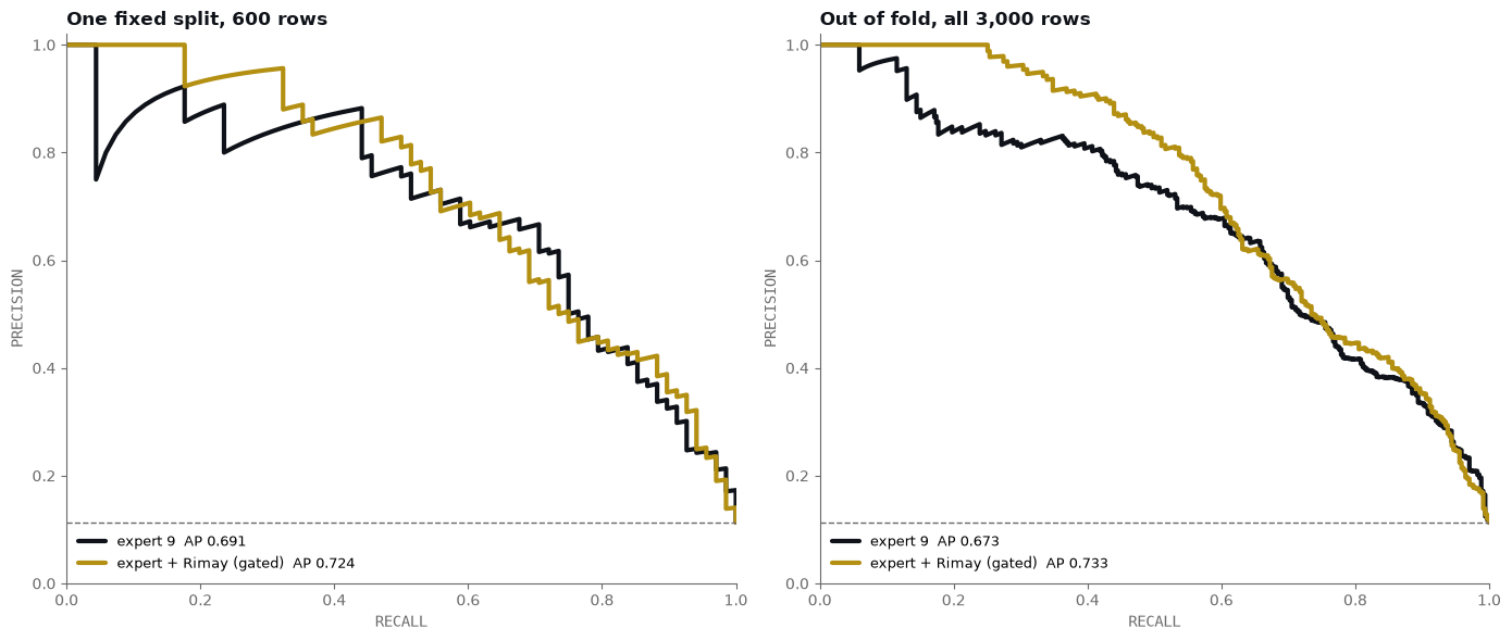
The staircases smooth out, and the gap holds and sharpens: +0.033 on the fixed split, +0.060 out of fold. The fixed split gave you one noisy draw of a quantity the out-of-fold reading pins down.
Pulling the steps together, this is what the measurements support and no more:
- The engineered physics is worth +0.0424 to +0.1163 average precision over the raw sensors for the three panel models. That step is real, significant, and involves nothing quantum.
- On top of the table that already carries the physics, the quantum columns add +0.0420 to +0.0582, significant under both protocols for all three models; the gate lifts naive Bayes to +0.0646. The study's stricter Holm reading of the naive Bayes cell is +0.0394 at p 6.1e-05.
- Quoted from the business session's own denied-arm extraction: quantum columns computed from the sensors alone moved no model significantly. The gain above is re-presentation of physics you sent, not discovery of physics you withheld.
- The study's two high-capacity models lose significantly on the same comparison (RBF SVM -0.0506, gradient boosting -0.0476), and gradient boosting on the engineered table alone reaches 0.9420 average precision, above every quantum arm.
None of that is a demonstration of quantum advantage. Every positive is AI4I, the only gainer of four datasets tested, on the free simulator tier. No QPU-backed Rimay evidence exists anywhere we can reach.
Outlook: the surrogate, or where the quantum computer goes
Everything you ran used the quantum stage at training time only, but retraining still needs the extraction, and on an on-premise or air-gapped plant floor a cloud round-trip is a policy violation. The surrogate answers that: while the quantum stage is available, train a small classical model to reproduce the extraction itself, and the whole pipeline then runs inside your own infrastructure. Kipu's off-line surrogate framework works the idea out: arXiv:2605.19801, or the shorter version on the blog. It is research with published results, not a button on the Hub, and nothing you measured depended on it.
The definition, extended
The business lesson gives the first three senses. The fourth is the one you built today: the extraction turned nine columns into seventeen without any new information entering, the models disagreed about what they are worth (three gaining, the study's two strongest losing), and the last two steps cost you real compute because a delta becomes a result only once it survives rows no model saw and a correction for everything you tried.
The protocol is now yours to run on a table of your own. Rimay sits on the Hub Marketplace with the same free tier, fifteen features and 3,000 rows. Session four looks at the Hub itself: the SDK, the CLI and MCP, and building your first hybrid quantum workflow as an API.
quan·tum ma·chine learn·ing
/ˈkwɒn.təm məˈʃiːn ˈlɜː.nɪŋ/noun
- 1
the use of a quantum processor somewhere inside a machine-learning pipeline, whether to represent the data, to fit the model, or to make the prediction.
- 2
Rimay is the tool that computes the re-presented fit-transform structure of your data so that a model can act on it.
Documentation: Kipu Quantum Hub | Hub docs | Quickstart | Service SDK | Using a service | Access tokens | Rimay product page | Rimay on the blog | Kipu Quantum Academy
Research: Quantum feature extraction on IBM hardware, MedMNIST and molecular toxicity (Scientific Reports 2026, doi:10.1038/s41598-026-67564-0) | Aerial tree-genus classification with quantum features (arXiv:2602.18350) | Off-line surrogate framework (arXiv:2605.19801) | Motor-imagery EEG classification, Carter et al., Mayo Clinic Proceedings 2026 | Heaton, an empirical analysis of feature engineering (arXiv:1701.07852) | Bengio, Courville and Vincent, representation learning (IEEE TPAMI 35(8), 1798 to 1828, 2013)